Basic operations
Simple example that introduce important concepts and functionality.
Potential surface with membrane
We want to calculate the electrostatic potential around a membrane protein. We need the structure of the protein, assign charges and radii (using the pdb2pqr tool), and create a low-dielectric slab that simulates the membrane. We then run apbs to solve the Poisson-Boltzmann equation and visualize the results.
PQR file
Have a PQR file for your membrane protein of interest available. Getting it from the Orientations of Proteins in Membranes database (OPM) is convenient because you can get a sense for the likely position of the membrane. In the following we assume we use the GLIC channel (a proton gated cation channel) with OPM/PDB id 3p4w as an example. Download the file from OPM and create the PQR file with pdb2pqr:
wget https://storage.googleapis.com/opm-assets/pdb/3p4w.pdb
pdb2pqr --ff CHARMM --whitespace --drop-water 3p4w.pdb 3p4w.pqr
Membrane position
The membrane will be simulated as a low-dielectric brick-shaped slab.
Obtain the boundaries of the membrane that OPM suggested: The file contains “DUM” atoms that show the position of the membrane surfaces. The protein is oriented such that the membrane is in the X-Y plane so we extract the minimum and maximum Z component of the DUM atoms using some Unix command line utilities:
grep '^HETATM.*DUM' 3p4w.pdb | cut -b 47-54 | sort -n | uniq
which gives
-16.200
 16.200
i.e., the membrane is located between -16.2 Å and +16.2 Å with a
thickness of 32.4 Å. The center of the membrane is at z = 0 and
the bottom is at z = -16.2.
Pore dimensions
Ion channels have aqueous pathways. They should be represented by a high dielectric environment that is also accessible to ions.
In order to add the pore regions we need to get approximate dimensions of the pore, which is represented as a truncated cone with a center in the X-Y plane and potentially differing radii at the top and bottom of the membrane plane.
You can run HOLE to get radii and positions.
For this tutorial we simply load the structure in a visualization tool
such a VMD, pymol or Chimera and
estimate a diameter of about 20 Å at the center of the protein, which
is at x=0 and y=0 in the plane of the membrane.
Set up run
Generate a template input file 3p4w.cfg for the protein:
apbs-mem-potential.py --template 3p4w.cfg
You only need to keep the sections
[environment][membrane][potential]
because everthing else is taken from your global configuration file
(~/.bornprofiler.cfg).
Edit the template in [environment] section and the set pqr file.
[environment]
pqr = 3p4w.pqr
Edit the template in the [membrane] section to add data for the
membrane.
lmemis the thickness, 32.4 Å; the membrane is set to a dielectric constant ofmdie.zmemis the bottom of the membrane,z=-16.2vmemis the cytosolic membrane potential (in ???); here we leave it at 0.headgroup_lis the thickness of the headgroup region with dielectric constantheadgroup_die. Here we keep it zero for simplicity, but if you have additional data you can set it to a non-zero value. (See, for example Fig 2c in [Stelzl2014]). The total membrane thickness is stilllmemand the hydrophobic core is thenlmem - 2*headgroup_l.- channel exclusion zone: a stencil with dielectric constant
cdie(by default, the solvent dielectric constant) in the shape of a truncated cone can be cut from the membrane. Its axis is parallel to the membrane normal and centered at absolute coordinatesx0_randy0_r. Alternatively, the center can be given relative to the center of geometry of the protein, with an offsetdx_randdy_r. The default is to position the exclusion zone at the center of the protein.
[membrane]
rtop = 10
rbot = 10
x0_r = None
y0_r = None
dx_r = 0
dy_r = 0
cdie = %(solvent_dielectric)s
headgroup_die = 20
headgroup_l = 0
mdie = 2
vmem = 0
lmem = 32.4
zmem = -16.2
The [potential] block sets the dimensions of the grid.
Run calculation
Once all information is collected in the cfg file, one runs
apbs-mem-potential.py 3p4w.cfg
This will create input files for apbs and run drawmembrane2a when necessary.
The output consists of dx files of the potential (in kT/e). Typically, these files a gzip-compressed to save space. For most external tools, uncompress them with gunzip.
In particular the following files are of interest:
- pot_membraneS.dx.gz: the potential on the grid in kT/e (calculated with membrane included)
- dielxSm.dx.gz: the dielectric map with membrane; visualize to verify that there are regions of different dielectric constants. (APBS needs maps that are shifted in X, Y, and Z; for visualization purposes, anyone is sufficient)
- kappaSm.dx.gz: map of the exclusion zone (with membrane)
- pot_bulksolventS.dx: the potential without a membrane (for comparison to see the effect of the membrane); other files without membrane have names similar to the afore mentione ones but without “m” as the last letter of the name before the .dx.gz.
Visualization
Uncompress the pot_membraneS.dx.gz file
gunzip pot_membraneS.dx.gz
and load the PQR file 3p4w.pqr (or the PDB file 3p4w.pdb) and
the DX file pot_membraneS.dx in your favorite visualization
tool. Contour the density at, for example, –5 kT/e and +5 kT/e.
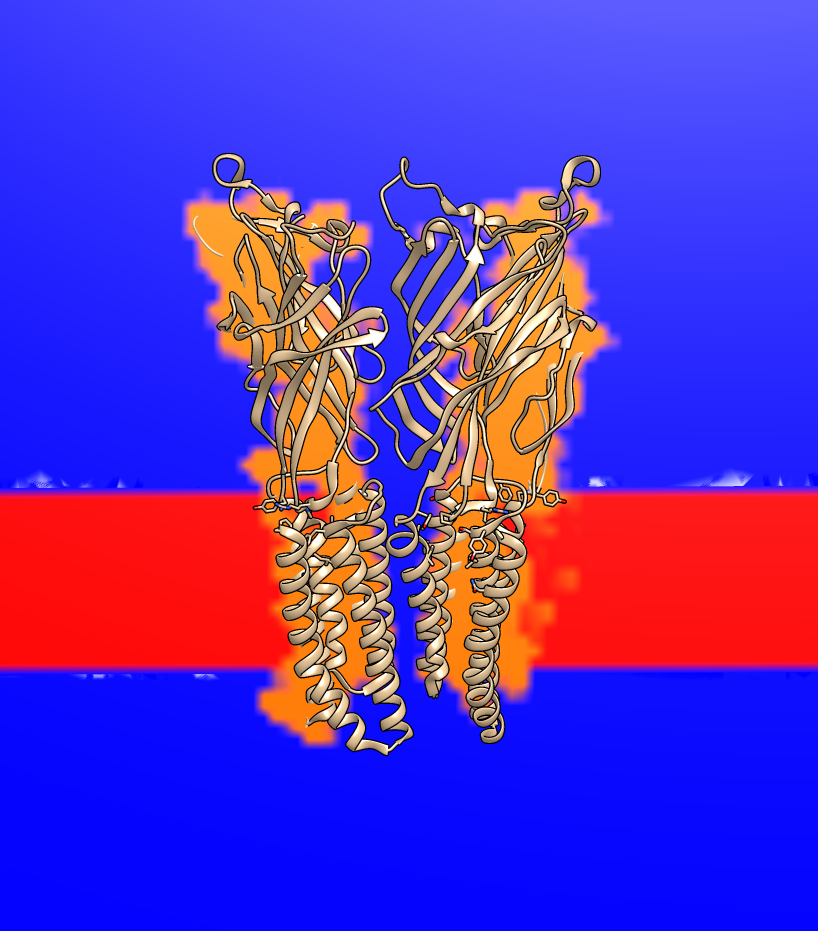
GLIC channel dielectric map dielxSm.dx visualized together with
3p4w.pdb. Epsilon 2 (membrane) is red, protein (10) is orange,
solvent (80) is blue. Visualized and rendered with UCSF Chimera.

GLIC channel electrostatic potential pot_membraneS.dx
visualized with the protein structure 3p4w.pdb. The potential
isocontour surface at –5 kT/e is shown in red, and the one at +5
kT/e in blue. The membrane dielectric region is shown as a gray
mesh. Visualized and rendered with UCSF Chimera.
A simple Born profile
TODO: Outline the problem of ion permeation, discuss simple example and show how this package can solve the problem. Choose something very simple such as nAChR or GLIC.